Advanced Lane Finding

Contents

1. Introdution
2. Data Samples
3. Requirements
4. Algorithm
5. Result
6. Challenges
7. Refernces

---

Introdution

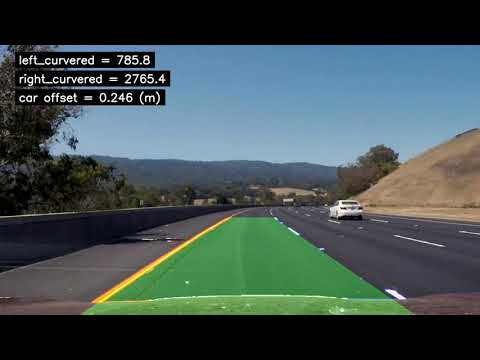
In this project, we will write a software pipeline to identify the lane boundaries in a video. The video was created from the centre camera. It also required to calculate the curvature of the road.

---

Data Samples

The test images are coloured with a resolution of 1280x720. The data is split into test images and three different videos with gradient difficulty. Blow a sample of images.

---

Requirements

This project is pure Python with a few depenendies

• OpenCV 1
• Numpy 2
• matplotlib 2

---

Algorithm

1. Compute the camera calibration matrix and distortion coefficients given a set of chessboard images.
2. Apply a distortion correction to raw images.
3. Use color transforms, gradients, etc., to create a thresholded binary image.
4. Apply a perspective transform to rectify binary image ("birds-eye view").
5. Detect lane pixels and fit to find the lane boundary.
6. Determine the curvature of the lane and vehicle position with respect to center.
7. Warp the detected lane boundaries back onto the original image.
8. Output visual display of the lane boundaries and numerical estimation of lane curvature and vehicle position.

1. Compute the camera calibration matrix

The code can be found on calibration.py

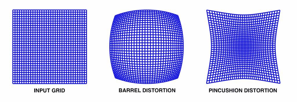
In this project, we will use a pinhole camera model4. Although the model is simple to use It comes with industrial defects. It can be called camera distortion5. Camera distortion is classified into two types.

Radial distortion	Tangential distortion
6	7

To overcome these distortions, We need to find a nonlinear equation which maps the distorted images into ideal image. This operation is called camera calibration. The camera calibration processes are a sequence of steps that try to reverse the camera distortion. The most common camera calibration is capturing several images for a checkerboard. Which will be passed to an optimization algorithm to find the distortion parameters. These parameters can be used to underscore the images.

The code for calibration is located on calibration.py file. We will use findChessboardCorners from OpenCV. which will get internal corners. The order of chekerboard corners in camera plane is welldefined. After getting 2d corner and predefined corner in camera plane we can use calibrateCamera from OpenCV too. Which will estimate camera matrix and camera distorition paramters.

ret, corners = cv2.findChessboardCorners(gray_image, grid_size, None)

2. Apply a distortion correction

Now can undistor the input camera, I select this two images because the ridal distortion is so clear in left side at undistort5 and in both sides of undistort1.

ret, mtx, dist, rvecs, tvecs = cv2.calibrateCamera(objpoints, imgpoints, gray_image.shape[::-1],None, None)

3. Binary thresholding

The code can be found on binary_thresholding.py

The code for calibration is located on binary_thresholding.py file. We need to isolate the lanes from the remaining of the image. We will use binary thresholding which means that anything passes the threshold we are set to one We need a combination of thresholding operation to isolate the lane lines.

Sobel9

is edge detection algorithms where it creates an image emphasising edges.

sobel_x = cv.Sobel(input_image, cv2.CV_64F, 1, 0, ksize=sobel_kernel)
sobel_y = cv.Sobel(input_image, cv2.CV_64F, 0, 1, ksize=sobel_kernel)

original	sobelx	sobely

1. SobelX and SobelY
2. Edge direction and magniture.
3. using Saturation channel from HLS color space.

At the thresholding stage. I used two strategies. First, I convert the input image from colour to grey and use grey in the remaining stages ie. I use grey for Sobel and combine the result with S channel from HLS colour space. Second, I convert the input image from colour to HLS colour space and use the S channel in the remaining stages.

TThe second approach is better except starting from frame number 1036. That's why I return to the first approach. I mention that again on the challenges part.

4. Apply a perspective transform

The code can be found on utilities.py

As shown in the next figure, I select fixed points on the input image which wrapped into the perspective view.

source_points = np.array([
    [270,  670], # Point 0
    [575,  460], # Point 1
    [740,  460], # Point 2
    [1100, 670]  # Point 3
], np.float32)

dest_points = np.array([
    [270,  670], # Point 0
    [270,  0],   # Point 1
    [1101, 0],   # Point 2
    [1100, 670]  # Point 3
], np.float32)

Prespective = cv2.getPerspectiveTransform(vertices, dest)

Before	After

5. Detect lane pixels

In this is the section we get deeper into the detection algorithm. The detection algorithm has two states. The code can be found on lane_detection.py

i. Not initialized or missing state The input image is a grey warped image. we take a histogram for the lower half of the image along the x-axis. That helps us find the estimated position of the lanes. Using the histogram peaks as shown in the next figure, we can get the x values for the left and right lanes. one step forward is to divide the image into several windows. In this project we use 9 windows. The window is used to estimate the number of pixels that is related to the lanes Divide and conquer. Iterate over windows while using the initially selected x-values to centralize the first window. using the window rectangle to select the white pixels. After selecting the left and right pixels, we can use polyfit function to estimate the polyline for the left and right lanes.

    lane_fit = np.polyfit(y, x, 2)

ii. Preinitialied Applying the last stages for every frame is a waste of time. The difference between frames should not be so big. We will use the last estimated lines to search for pixels on the new image. After finding the pixels for both lanes run polyfit function again. And use the new lines.

6. Determine the curvature

The code can be found on lane_detection.py under Lane_Manager

7. Warp the detected lane boundaries

The code can be found on main.py

---

Result

---

Youtube

---

Challenges

• I used to convert the colour image to different colour spaces HLS,HSV,LAB and understand the difference.

• Using the S channel as a source for binary thresholding. It generates more clear binary output better than grey still It can be affected by noise at the end of the first video.

	color	gray	s_channel	combined
Normal
Noise

---

Refernces

1. https://opencv.org/
2. https://numpy.org/
3. https://matplotlib.org/
4. https://en.wikipedia.org/wiki/Pinhole_camera
5. https://en.wikipedia.org/wiki/Distortion_%28optics%29
6. https://learnopencv.com/understanding-lens-distortion/
7. Evaluation of a Bisensor System for 3D Modeling of Indoor Environments
8. https://opencv-python-tutroals.readthedocs.io/en/latest/py_tutorials/py_calib3d/py_calibration/py_calibration.html
9. https://en.wikipedia.org/wiki/Sobel_operator